Dragonfly Help > Image Processing > Image Filters and Settings

Image Filters and Settings

Image filtering is one of the most fundamental operations of image processing and can greatly improve image quality and yield information that otherwise would have been missed. You should note that some filters are known for detecting or preserving edges, while others are typically used for smoothing or denoising. You should also note that filter performance is dependent both on the input image and on the parameters selected for filtering, such as kernel shape and size, iterations, and interpretation.

Sometimes the best results may be obtained by applying two or more filters sequentially. For example, you may need to preserve edges while smoothing uniform yet noisy areas. In the Image Processing panel, you can simply add sequential filtering operations to create a composite filter. However, you should be careful to note your order of operations as some filters may be contradictory and may not always be simply applied sequentially.

A number of image filters and image processing algorithms can be performed either on each XY-slice of the volume using a 2D kernel or on the whole volume using a 3D kernel. In some cases, it may be preferable to interpret the input data of an image processing algorithm as a sequence of 2D planes, either for performance or for a more appropriate outcome.

You can also easily create your own specialized filters with the Simple Dataset Filter Generator (see Generating Simple Dataset Filters). You can also browse for and download filters in the Infinite Toolbox (see Infinite Toolbox).

The tables below provide descriptions and the settings for the standard image filters available in Dragonfly and Dragonfly Pro. These filters are grouped in categories for easy reference.

Artifact Removal

These filters can be used to remove vertical and horizontal stripes, as well as stripes that appear in any direction, from image data. The destriping filters work by adding a pattern that interferes with the image to remove stripes, as shown in the example below for vertical destriping.

Original data (below left) and preview after destriping (below right)

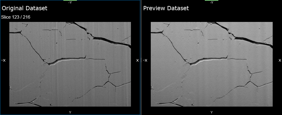
These filters are often used to correct artifacts found on FIB-SEM acquired data.

Artifact removal filters and settings
	Type	What it does	Settings
Arbitrary Angle Destriping	2D	Removes stripes that appear at an arbitrary angle, using the Fourier-Wavelet based method.	Angle Sigma foreground Sigma background Levels Wavelet
Horizontal Destriping	2D	Removes horizontal stripes, using the Fourier-Wavelet based method.	Sigma foreground Sigma background Levels Wavelet
Vertical Destriping	2D	Removes vertical stripes, using the Fourier-Wavelet based method..	Sigma foreground Sigma background Levels Wavelet

Contrast

These filters can be used to adjust the contrast in images by remapping the grayscale or by recalculating the range of values in an image.

Contrast adjustment filters and settings
	Type	What it does	Settings
CLAHE	2D	A variant of adaptive histogram equalization, CLAHE (contrast limited adaptive histogram equalization), prevents a tendency to over amplify noise in relatively homogeneous regions of an image by limiting amplification. In the case of CLAHE, the contrast limiting procedure is applied for each neighborhood from which a transformation function is derived.	Clip Nb tiles Bins
Histogram Equalization	2D	Remaps image intensities so that the output image uses the entire range available and there are approximately the same number of pixels of each value in the output image.	- -
Local Histogram Equalization	2D	Enhances images with low contrast by spreading out the most frequent intensity values.	Kernel size
Normalization	2D	Recalculates the range of pixel values in an image so that it is equal to the maximum range for the data type. The purpose of this dynamic range expansion is usually to bring the image, or other type of signal, into a range that is more familiar or normal.	- -
Slope Map	2D	Relies on the blurring effects of a Gaussian filter to quantify underlying local trends characterizing image intensity and balance contrast. This filter can remove vignetting artifacts quite effectively.	Scale

Detector

These filters emphasize the edges and transitions in an image.

Detector filters and settings
	Type	What it does	Settings
Frangi Filter	2D	Typically used to detect vessel-like or tube-like structures and fibers in volumetric image data.	- -
Frangi Filter	3D	Typically used to detect vessel-like or tube-like structures and fibers in volumetric image data.	Standard deviation Output Filter
Hessian	2D	Finds continuous edges in an image. Almost equal to the Frangi filter, this filter is implemented with an alternative method for smoothing.	- -

Edge Detection

These filters emphasize the edges and transitions in an image.

Edge detection filters and settings
	Type	What it does	Settings
Canny	2D	Emphasizes the edges in an image using the Canny algorithm.	Sigma
DoG (Difference of Gaussian)	2D	Performs a Gaussian blur on an image at a specified standard deviation (first sigma). The resulting image is a blurred version of the source image. The module then performs another blur that blurs the image less than previously (second sigma). The final image is then calculated by replacing each pixel with the difference between the two blurred images and detecting when the values cross zero. The resulting zero crossings will be focused at edges or areas of pixels that have some variation in their surrounding neighborhood.	First sigma Second sigma Normalized
Laplacian	2D/3D	The Laplacian filter highlights the regions in which there is a rapid intensity change using a discrete convolution kernel that approximates the second derivatives of the image in the definition of the Laplacian.	2D or 3D kernel
Prewitt	2D	Finds the horizontal and/or vertical edges of an image using the Prewitt transform.	Direction (combined, vertical, or horizontal)
Scharr	2D	Finds the horizontal and/or vertical edges of an image using the Scharr transform.	Direction (combined, vertical, or horizontal)
Sobel	2D/3D	Emphasizes edges and transitions in an image.	2D or 3D kernel

Editable

Lets you create your own filter effects — smoothing, sharpening, intensifying, enhancing — with a customized 2D or 3D kernel for convolution.

Editable filters and settings
	Type	What it does	Settings
Editable Filter	2D/3D	Convolves an image with a customized 2D or 3D kernel, which lets you create filter effects such as smoothing, sharpening, intensifying, enhancing.	Kernel shape and size

Frequency Domain

Two filters — Discrete Fourier Transform and Inverse Discrete Fourier Transform — are available for transforming time domain signals to the frequency domain and for inverting transformed signals.

The perfect invert-ability of the Discrete Fourier Transform is an important property for building filters which remove noise or particular components of a signals spectrum. Although frequency artifacts can be common in the result of a Fourier transform, these artifacts do not result in error in the inverted signal.

Frequency domain filters
	What it does
Discrete Fourier Transform	The Discrete Fourier Transform (DFT) takes a signal in the so-called time domain (where each sample in the signal is associated with a time) and maps it, without loss of information, into a frequency domain series, where each value is a complex number that is associated with a given frequency. The outputs of the DFT are the magnitude and phase information, as well as the real (even) and imaginary (odd) parts of the transform.
Inverse Discrete Fourier Transform	The Inverse Discrete Fourier Transform (IDFT) takes the frequency series of complex values and maps them back into the original time series. Assuming that the original time series consisted of real values, the result of the IDFT will be complex numbers where the imaginary part is zero. The required inputs of the IDFT are the magnitude and phase information.

Information

Information filters and settings
	Type	What it does	Settings
Entropy	2D	Detects subtle variations in the local gray level distribution.	Disk Normalized

Morphology

Morphological operators — dilate, erode, open, and close — can be applied through image filtering to grow or shrink image regions, as well as to remove or fill-in image region boundary pixels.

Morphology filters and settings
	Type	What it does	Settings
Black Top Hat	2D/3D	Returns an image containing the objects or elements of the input image that are smaller than the structuring element and darker than their surroundings (see also Top Hat Filters).	Kernel shape and size
Close	2D/3D	Performs a dilation operation, followed by erosion to smooth objects and fill in small holes.
Dilate and Erode	2D/3D	Enlarges the boundaries of regions of foreground pixels, typically white pixels.
Dilate and Erode	2D/3D	Erodes away the boundaries of regions of foreground pixels, typically white pixels.
Morphological Gradient	2D/3D	Produces an image where each pixel value indicates the contrast intensity in the close neighborhood of that pixel.
Morphological Laplace	2D/3D	Enhances the edges of an image. The morphological Laplacian can be defined as half the sum of a morphological dilation and a morphological erosion with the same structuring element, minus the original image.
Open	2D/3D	Performs an erosion operation, followed by a dilation to smooth objects and remove isolated pixels.
White Top Hat	2D/3D	Returns an image containing objects or elements of the input image that are smaller than the structuring element and brighter than their surroundings. See also Top Hat Filters.

Segmentation

These filters — K-Means and Mini-Batch K-Means — can be used to partition an image into a specific number of meaningful regions.

Original data (below left) and preview after clustering (below right)

Segmentation filters and settings
	Type	What it does	Settings
K-Means	2D/3D	Clusters data by trying to separate samples in n groups of equal variance, minimizing a criterion known as the inertia or within-cluster sum-of-squares. This algorithm requires the number of clusters to be specified. Refer to https://scikit-learn.org/stable/modules/clustering.html for more information about K-Means clustering.	Initialization Number of K Iterations
Mini-Batch K-Means	2D/3D	The Mini-Batch K-Means option is a variant of the K-Means algorithm which uses mini-batches to reduce computation times, while still attempting to optimize the same objective function. Mini-batches are subsets of the input data, randomly sampled in each training iteration. In contrast to other algorithms that reduce the convergence time of K-Means, Mini-Batch K-Means produces results that are generally only slightly inferior to the standard algorithm. Refer to https://scikit-learn.org/stable/modules/clustering.html for more information about this variation of the K-Means clustering.	Initialization Number of K Iterations Batch size

Shading Compensation

These filters can be used to correct undesirable shading across the field-of-view, which can be a prominent phenomenon in microscopy and may occur due to non-uniform illumination, inhomogeneous detector sensitivity, or non-specific sample staining,

Shading compensation filters and settings
	Type	What it does	Settings
Histogram Balancing	2D	Spreads out the most frequent intensity values in an image. The equalized image has a roughly linear cumulative distribution function.	Reference slice
Local Entropy Minimization *	2D	Corrects non-uniform illumination and counteracts noise by reducing randomness.	Node count and Iteration Count Compensation
Manual RBF*	2D	Uses a radial basis function to correct image shading. You should note that the Manual RBF filter requires at least three(3) seed points in representative regions and that corrections are applied in the X and Y axes only. If corrections are required in another direction, you will need to transform the data (see Inverting Datasets).	Kernel size Compensation Sampling points (at least 3)
Polynomial	2D	Uses a third degree polynomial to correct uneven shading.	Polynomial degree Compensation

* Available only for Dragonfly Pro. Contact Object Research Systems (ORS) Inc. for information about the availability of Dragonfly Pro.

Sharpening

These filters can be used to emphasize the details in an image and enhance the edges of objects.

Sharpening filters and settings
	Type	What it does	Settings
Gaussian High Pass	2D/3D	Effectively blurs or smoothes images by allowing high frequency image information to pass through and blocking low frequency image information. This effectively sharpens the image.	Kernel size Standard deviation
Unsharp	2D/3D	Sharpens an image by subtracting a blurred version of itself from the original.	Kernel size Standard deviation Unsharp factor

Smoothing

These filters can be applied to reduce the amount of noise in an image.

Smoothing filters and settings
	Type	What it does	Settings
Anisotropic Diffusion	2D	Anisotropic diffusion is a generalization of this diffusion process as it produces a family of parameterized images, but each resulting image is a combination between the original image and a filter that depends on the local content of the original image. As a consequence, anisotropic diffusion is a non-linear and space-variant transformation of the original image. Anisotropic diffusion generally preserves the sharpness of edges better than Gaussian blurring.	Option K Iterations
Bilateral	2D	This edge-preserving and noise reducing denoising filter averages pixels based on their spatial closeness and radiometric similarity.	Sigma color Sigma spatial
Gaussian	2D/3D	Smoothes or blurs an image by performing a convolution operation with a Gaussian filter kernel.	Kernel size Standard deviation
Kuwahara	2D	Provides non-linear smoothing for adaptive noise reduction. Most filters that are used for smoothing are linear low-pass filters that effectively reduce noise, but can also blur out the edges. However, the Kuwahara filter is usually able to apply smoothing on the image while preserving its edges.	Kernel size
Maximum	2D/3D	Replaces each pixel in the image with the largest pixel value in that pixel’s neighborhood. This grayscale dilation can help reduce pepper noise.	Kernel shape and size
Mean	2D/3D	Smoothes images and diminishes noise by replacing each pixel with the mean value of its neighbors.	Kernel shape and size
Mean Shift	2D	Mean shift filtering is based on a data clustering algorithm commonly used in image processing and can be used for edge-preserving smoothing,	Kernel size Maximal distance X and Y Noise spread
Median	2D/3D	Smoothes images by replacing each pixel with the median value of its neighbors. Can be very effective on salt-and-pepper noise, without the smoothing effects that can occur with other smoothing filters.	Kernel shape and size
Minimum		Replaces each pixel in the image with the smallest pixel value in that pixel’s neighborhood. This grayscale erosion can help reduce salt noise.	Kernel shape and size
Non-Local Means*	2D/3D	Smoothes images by taking a mean of all pixels, weighted by how similar the pixels are to the target pixel.	Kernel size Smoothing Rician noise
Percentile	2D/3D	Percentile filtering is a well known non-linear technique for filtering images in which each pixel in the image is replaced by the value of that point in the histogram of its neighbour pixels that corresponds with a selected percentile. Percentile filtering includes minimum and maximum filtering (grey-value erosion and dilation) and median filtering. It is very suitable for background estimation and removal of outliers without degrading the image. NOTE The median filter corresponds to the case where the percentile selected is 50.	Kernel shape and size Percentile value
Rank	2D/3D	Is a non-linear local filter that proceeds by ordering the pixels in a neighborhood and selecting a given ranked entry.	Kernel shape and size Rank value
Tv_bregman	2D/3D	Performs total-variation denoising using a split-Bregman optimization. Total-variation denoising minimizes the total variation of an image, which can be roughly described as the integral of the norm of the image gradient. Refer to http://en.wikipedia.org/wiki/Total_variation_denoising for more information about the principle of total-variation denoising.	Weight Max iterations Isotropic
Tv_chambolle	2D/3D	Performs total-variation denoising on n-dimensional images. NOTE The code for the Tv_chambolle filter is an implementation of the algorithm of Rudin, Fatemi and Osher that was proposed by Chambolle in An algorithm for total variation minimization and applications, Journal of Mathematical Imaging and Vision, Springer, 2004, 20, 89-97.	Weight Max iterations
Wavelet	2D	Performs a wavelet transform, using the selected wavelet function, which is characterized by a width parameter and length parameter.	Wavelet Mode

* Available only for Dragonfly Pro. Contact Object Research Systems (ORS) Inc. for information about the availability of Dragonfly Pro.

Texture Analysis

Texture analysis characterizes the texture of a region by quantifying spatial variation in pixel intensities.

Texture analysis filters and settings
	What it does	Settings
Gabor	Separates elements with oriented patterns.	Frequency Theta
Image Moments	Separates elements with different textures.	Kernel Order
Local Binary Pattern	Separates elements with different textures.	Angular count Radius Method
Membrane Projections	Enhances membrane-like structures of an image through directional filtering.	Kernel size Projection type Number of angles

Thresholding

Thresholding filters output an image composed of two basic classes — foreground and background. These images can be used as masks for segmentation purposes or for other image processing tasks.

Thresholding filters and settings
	What it does	Settings
Adaptive	Applies an adaptive threshold to images.	Kernel size
Adaptive Gaussian	The threshold value is the weighted sum of neighbourhood values where weights are a Gaussian window.	Threshold type Block size Constant
Isodata	Return threshold value(s) based on ISODATA method. That is, returned thresholds are intensities that separate the image into two groups of pixels, where the threshold intensity is midway between the mean intensities of these groups.	- -
Li	Implements Li's Minimum Cross Entropy thresholding method.	- -
Local Otsu	Performs local Otsu thresholding on an image, with a user-specified kernel size. Facilitates the threshold-segmentation of images with uneven illumination, without the need for background normalization, and for which global thresholding is inadequate.	Kernel size
Mean	Selects the threshold as the mean of the local greyscale distribution.	- -
Minimum	Selects the threshold as the minimum of the local greyscale distribution.	- -
Niblack	Applies a Niblack local threshold to an array. Instead of calculating a single global threshold for the entire image, several thresholds are calculated for every pixel by using specific formulae that take into account the mean and standard deviation of the local neighborhood (defined by a window centered around the pixel). NOTE Refer to Niblack, W (1986), An introduction to Digital Image Processing, Prentice-Hall for more information.	Window size k
Otsu	Otsu's threshold clustering algorithm searches for the threshold that minimizes the intra-class variance, defined as a weighted sum of variances of the two classes.	- -
Sauvola	Uses a modification of the Niblack technique.	Window size k
Triangle	Returns a threshold value based on the triangle algorithm.	- -
Yen	Implements Sauvola's thresholding method, which is a variation of Niblack's method.	- -

	Video Tutorials \| www.theobjects.com/dragonfly/tutorials.html
	Recorded Webinars \| www.theobjects.com/dragonfly/learn-recorded-webinars.html

	Forums \| www.theobjects.com/dfforums/index.php
	Technical Support \| www.theobjects.com/dragonfly/gethelp.html